The Shape of Thought: Space Folding in Neural Networks
The mathematical description of deep learning has long been dominated by the language of algebra: matrices, gradients, and optimization landscapes. A parallel and perhaps more intuitive language however is emerging, one of geometry and topology. In this view, a neural network is not merely a function approximator but a complex geometric operator that manipulates the very fabric of the input space. It stretches, twists, and, crucially, folds high-dimensional manifolds to disentangle information. Over the past year I collaborated with Michał Lewandowski and others, in order to understand, measure and exploit this notion of space folding in neural networks.
We published our thoughts and findings in a series of quite foundational papers, and in this post I'll try to give you a thorough overview of the idea of Space Folding, as well as ideas from our papers that you hopefully find helpful or interesting.
Current theoretical frameworks posit that the success of deep learning arises from its ability to disentangle complex data manifolds. The "Manifold Hypothesis" suggests that real-world data (e.g. images, audio, text) lies on low-dimensional surfaces embedded within high-dimensional space. The "black box" of the neural network operates by continuously transforming this space until the data manifolds are flattened and linearly separable. While this topological perspective has been discussed qualitatively for years, recent innovations have allowed for its rigorous quantification.
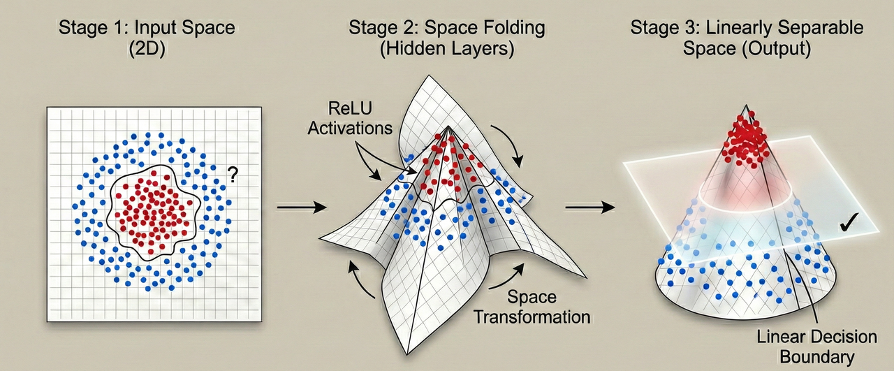
By analyzing the specific mechanics of how neural networks map straight lines in the Euclidean input space to trajectories in the internal activation space, we uncover a process analogous to the ancient art of origami. The network learns to crease and fold the input space, effectively bringing distant points together and pushing adjacent points apart to form decision boundaries.
To visualize the fundamental intuition behind space folding before descending into the rigorous mathematical analysis, consider the following visualization:
In this blogpost I will dissect the mathematical construction of the Space Folding Measure ($\chi$), its generalization to non-ReLU architectures via Equivalence Classes, the algorithmic challenges of sampling high-dimensional folds, and the profound implications of folding for generalization and adversarial robustness.
Part I: Foundations of Activation Space Geometry
To understand the mechanism of space folding, one must first establish the geometric environment in which neural networks operate. The transformation from raw input to abstract representation is defined by the mapping between two distinct metric spaces: the continuous Euclidean space of the input and the discrete Hamming space of the neuron activations.
The Manifold Hypothesis and Topological Entanglement
The Manifold Hypothesis is the bedrock of geometric deep learning. It asserts that high-dimensional data is not uniformly distributed but is concentrated near a lower-dimensional manifold. For example, the space of all possible $28 \times 28$ pixel grids is $\mathbb{R}^{784}$, but the subset of grids that look like handwritten digits occupies a tiny, highly structured sub-manifold within that space.1
In a classification task, different classes (e.g., digits "0" and "1") occupy disjoint manifolds. However, in the raw input space, these manifolds are often hopelessly entangled and twisted around each other like two crumpled sheets of paper compressed into a ball. A linear classifier (a single flat hyperplane) cannot separate them because any planar cut would intersect both manifolds.
Deep neural networks solve this problem through a sequence of layer-wise transformations. Each layer acts as a homeomorphism (or near-homeomorphism), effectively "uncrumpling" the paper. By the final layer, the manifolds are flattened and separated, allowing a simple linear readout to classify the data. The "Space Folding" theory argues that this uncrumpling is achieved not just by stretching, but by recursive folding operations that simplify the topological complexity of the data.
The Crumpled Paper Analogy
The metaphor of crumpled paper is ubiquitous in the study of disordered systems and serves as a potent analog for the neural network's internal state.5
- The Unfolded State (Target): The goal of the network is to produce a representation where the data is organized as simply a flat sheet of paper where "zeros" are on the left and "ones" are on the right.
- The Crumpled State (Input): The input data is the crumpled ball. Points that are far apart on the flat sheet (geodesically distant) may end up touching in the crumpled ball (Euclidean proximity). Conversely, points that are close on the sheet might be separated by a fold.
- The Folding Operator: The neural network learns the inverse operation. It learns where the creases are. By identifying the folds and reversing them, it recovers the underlying structure of the data.
Crucially, the "ridges" or creases in a crumpled sheet carry the majority of the structural information. Similarly, in a neural network, the "Linear Regions" (the so-called "polytopes" created by the activation functions) are defined by the boundaries where neurons switch from inactive to active. Investigating these boundaries reveals the "bulk" geometry of the network's knowledge.
ReLU Networks as Piecewise Affine Transformations
The Rectified Linear Unit (ReLU), defined as $\sigma(x) = \max(0, x)$, is the primary driver of this analysis in modern deep learning. Geometrically, a single ReLU neuron creates a hyperplane cut in the input space.
- Active Half-Space ( $x > 0$ ): The neuron behaves linearly. The space is preserved (though potentially rotated or scaled by weights).
- Inactive Half-Space ( $x \leq 0$ ): The neuron outputs zero. The space is collapsed or "folded" onto the hyperplane boundary.
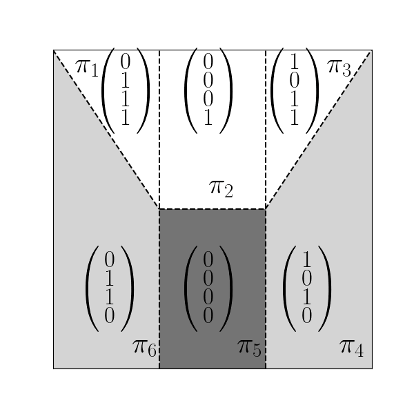
When $N$ neurons are combined in a layer, they partition the input space into a convex polyhedron. When $L$ layers are stacked, these partitions compound, creating a complex tessellation of the input space into Linear Regions. Within each region, the network is purely affine (linear). However, the global function is highly non-linear, with sharp "creases" at the boundaries of these regions.
Early theoretical work focused on counting these regions as a proxy for expressivity. A deep network can generate exponentially more linear regions than a shallow network with the same number of neurons. However, counting regions ignores their arrangement. The Space Folding theory argues that the topology of these regions, i.e how they are folded back onto each other, is the true driver of representation learning.
Part II: Quantifying the Fold – The Measure $\chi$
While the qualitative description of neural networks as folding operators has existed for over a decade (e.g., Montúfar et al., 2014), quantifying this phenomenon has remained a significant challenge. Our paper introduces the first rigorous metric to measure this folding effect: the Space Folding Measure $\chi$.
The Theoretical Conflict of Convexity
The derivation of $\chi$ begins with a fundamental observation about the preservation (or loss) of convexity when mapping between spaces.
Consider two points $x_1$ and $x_2$ in the Euclidean Input Space ($\mathcal{X}$). The shortest path between them is a straight line segment. This segment is inherently convex; every point on the line is a weighted average of the endpoints.
Now, consider the mapping of this line into the Hamming Activation Space ($\mathcal{H}$). The activation pattern of the network is a binary vector $\pi(x) \in {0, 1}^N$, representing the state of all neurons (1 for active, 0 for inactive). The distance metric in this space is the Hamming distance $d_H$ (the number of differing bits).
The Convexity Lemma:
Research proves a critical equivalence: A union of activation regions in the input space is convex if and only if the corresponding set of activation patterns is convex in the Hamming space.
This lemma has a profound implication: Folding is impossible in a single layer. A single layer of ReLU neurons creates a convex partition (a Voronoi-like tessellation). A straight line in the input space maps to a "straight" path in the activation space of the first layer. The Hamming distance from the origin increases monotonically.
Folding emerges only with depth. The second layer acts on the partitions of the first, effectively grouping non-adjacent regions and mapping them to similar outputs. This destroys the convexity of the path. A straight line in the input space, when mapped through a deep network, becomes a curved, looping trajectory in the activation space.
Construction of the Measure $\chi$
The Space Folding Measure $\chi$ quantifies this deviation from convexity. It is constructed using range metrics adapted from the theory of random walks.
Consider a straight path $\Gamma$ in the input space connecting $x_1$ and $x_2$. This path is discretized into steps, producing a sequence of activation patterns ${\pi_1, \pi_2, \dots, \pi_n}$ in the Hamming space.
We compute two range metrics for this path:
- Maximum Net Displacement ($r_1$): This represents the furthest "distance" the path reaches from its starting point in the activation space. $$r_1(\Gamma) = \max_{i} d_H(\pi_i, \pi_1)$$ If the space is flat (unfolded), every step takes the path further away, so the maximum distance is simply the distance to the end point.
- Total Path Length ($r_2$): This is the cumulative sum of all steps taken along the path. $$r_2(\Gamma) = \sum_{i=1}^{n-1} d_H(\pi_i, \pi_{i+1})$$ This represents the total "energy" or "effort" expended to traverse the path.
The Definition:
The Space Folding Measure $\chi(\Gamma)$ is defined as the normalized deficit between the net displacement and the total length:
$$\chi(\Gamma) = 1 - \frac{r_1(\Gamma)}{r_2(\Gamma)}$$
Interpretation and Bounds
The measure is normalized such that:
- $\chi(\Gamma) = 0$ (The Flat Condition):
If the network has not folded the space along this path, then every step moves the activation pattern further from the start. $r_1$ (max distance) equals $r_2$ (total distance). The ratio is 1, and $\chi = 0$. This indicates a preservation of convexity; the straight line remains "straight" in the high-dimensional representation. - $\chi(\Gamma) > 0$ (The Folded Condition):
If the network folds the space, the path will loop back. The sequence of activations might look like $A \to B \to C \to B \to A$. In this case, the total path length ($r_2$) is 4 steps, but the maximum displacement ($r_1$) is only 2 steps (to C). $\chi = 1 - 2/4 = 0.5$. This indicates that points $x_1$ and $x_5$ are far apart in Euclidean space but identical in Activation space and therefore a perfect fold. - $\chi(\Gamma) \to 1$ (The Infinite Loop):
In a theoretical limit where a path oscillates infinitely between two adjacent regions without ever moving away, $r_2 \to \infty$ while $r_1$ remains constant. $\chi$ approaches 1. While rare in practice, this represents a "black hole" of folding where infinite input variation maps to finite activation outputs.
Mathematical Properties of $\chi$
Rigorous analysis has established several key properties of this measure, confirming its suitability as a robust geometric metric:
1. Stability:
Multiple steps taken within the same linear region do not affect $\chi$. Since the Hamming distance between identical patterns is 0, neither $r_1$ nor $r_2$ increases. This ensures that the measure is invariant to the sampling resolution, provided the resolution is fine enough to catch all region boundaries.
2. Asymmetry:
The measure is sensitive to direction. $\chi(\Gamma_{A \to B})$ is not necessarily equal to $\chi(\Gamma_{B \to A})$.
Intuition: Folding a piece of paper is mechanically different from unfolding it. Traversing "down" a fold (compressing space) might yield different activation dynamics than traversing "up" (expanding space). This asymmetry reflects the directed nature of the information processing pipeline in feedforward networks.
3. Flatness Invariance:
While the value of folding may differ directionally, the state of being flat is invariant. If a path is flat ($\chi=0$) in one direction, it is mathematically guaranteed to be flat in the reverse direction.
4. Non-Additivity:
The folding measure of a concatenated path $\Gamma_1 \oplus \Gamma_2$ is not the sum of its parts.
$$\chi(\Gamma_1 \oplus \Gamma_2) \neq \chi(\Gamma_1) + \chi(\Gamma_2)$$
This property is crucial. It implies that folds interact. A fold in the second segment might cancel out a fold in the first segment (unfolding), or it might compound it (double folding). This interaction is later defined as the Interaction Coefficient $\mathcal{I}$.
Part III: Generalizing the Fold – Beyond ReLU
The initial formulation of Space Folding relied on the discrete linear regions created by ReLU activations. However, the landscape of deep learning is diverse, utilizing activation functions like Swish, GELU, Sigmoid, and Tanh, which are continuous and curved. These functions do not partition space into discrete linear polytopes, theoretically rendering the definition of "Linear Regions" void.
To address this, we propose a significant innovation: the generalization of activation patterns via Equivalence Classes.
The Limits of Linear Regions
In a strict ReLU network, a linear region is a set of inputs sharing the exact same binary activation pattern. Inside this region, the derivative is constant. For a curved function like Sigmoid, the output is never strictly constant; it varies continuously. There are no "regions" of constant linearity.
However, the geometric intuition of folding/partitioning space into "active" and "inactive" zones remains.
Innovation: Equivalence Classes via Pre-Images
The authors observe that any monotonic continuous activation function $f$ can essentially partition the input domain into two connected sets based on a threshold (typically 0).
- Set A (Inactive/Negative): The pre-image $f^{-1}((-\infty, 0])$.
- Set B (Active/Positive): The pre-image $f^{-1}((0, \infty))$.
Using this observation, we can define a generalized Activation Pattern $\pi(x)$ for any network. $\pi(x)$ is a binary vector where the $i$-th bit is determined by which set the input falls into for the $i$-th neuron.
$$
\pi(x)_i = \begin{cases}
1 & \text{if } f(z_i(x)) > 0 \\
0 & \text{if } f(z_i(x)) \leq 0
\end{cases}
$$
Definition of Equivalence:
Two inputs $x_1$ and $x_2$ are defined as being in the same Equivalence Class if they map to the same binary activation pattern:
$$
x_1 \sim_{\mathcal{N}} x_2 \iff d_H(\pi(x_1), \pi(x_2)) = 0
$$
This elegant redefinition decouples the Space Folding Measure from the specific mechanics of ReLU. Whether the activation is a sharp corner (ReLU) or a smooth curve (Swish), the input space is still partitioned into equivalence classes. A "fold" is now rigorously defined as a traversal across the boundaries of these classes that results in non-monotonic distance changes. This allows $\chi$ to serve as a universal metric for neural geometry.
Part IV: The Algorithmic Challenge – Adaptive Sampling
Calculating $\chi$ effectively requires computing the path length $r_2$, which involves summing the Hamming distances between consecutive points on the path. This presents a massive computational challenge: Sampling.
The Failure of Equidistant Sampling
A naive approach would be to sample $N$ points equidistantly along the line segment $[x_1, x_2]$. This fails for two reasons:
- Oversampling (Redundancy): In large linear regions (e.g., describing the background of an image), the activation pattern might not change for a long distance. Thousands of equidistant samples might fall into the same class, wasting computation on $\delta=0$ steps.
- Undersampling (Aliasing): Near the decision boundaries, the linear regions can become microscopically thin. A fixed step size might "jump" over a region entirely. If the path jumps from Region A to Region C, missing Region B, the Hamming distance calculation becomes corrupted (e.g., recording a distance of 2 instead of $1+1$). This creates errors in $r_2$ and leads to an incorrect $\chi$.
Innovation: Adaptive Hamming Sampling
To solve this, we came up with a Parameter-Free Adaptive Sampling Strategy that operates based on topological feedback rather than Euclidean distance.
The Algorithm:
The algorithm dynamically adjusts the step size $\Delta t$ based on the observed change in Hamming distance.
- Initialize: Start at $x_{curr} = x_1$ with an initial step size $\Delta t$.
- Propose Step: Calculate a candidate point $x_{next} = x_{curr} + \Delta t \cdot \vec{d}$.
-
Check Topology: Compute the activation pattern $\pi_{next}$ and the Hamming distance $\delta = d_H(\pi_{curr}, \pi_{next})$.
- Case $\delta = 0$ (Stable): The step is within the same equivalence class. The topology is flat locally. We can potentially increase $\Delta t$.
- Case $\delta = 1$ (Ideal): We have crossed exactly one boundary (a facet). This is the atomic unit of folding. Record the step, update $x_{curr}$ to $x_{next}$.
-
Case $\delta > 1$ (Overshoot): We have crossed multiple boundaries at once or jumped a region. The step size is too large to resolve the local geometry. Refine: Halve the step size ($\Delta t \leftarrow \Delta t / 2$) and retry.
-
Loop: Continue until $x_2$ is reached.
Complexity Analysis:
The computational cost of this algorithm is $O(n \cdot (N+C))$, where $N$ is the number of neurons and $C$ is the inference cost. By ensuring that every single boundary crossing is detected (Hamming distance of 1), the algorithm guarantees the topological accuracy of the measure while minimizing redundant forward passes in empty space. This makes the calculation of $\chi$ feasible even for deep, high-dimensional networks.
Part V: The Geometry of Generalization
Why does space folding matter? Is it merely a geometric curiosity, or does it correlate with the fundamental performance metrics of AI? Extensive empirical evaluation on datasets like MNIST and CIFAR-100 reveals a compelling link: Folding is the engine of Generalization.
Folding Increases with Learning
By tracking the Global Folding Measure $\Phi_{\mathcal{N}}$ (the median $\chi$ across random paths) throughout the training process, we observed a monotonic relationship.
- Initialization: At initialization (random weights), the network exhibits some baseline folding due to random hyperplanes.
- Training: As the network learns and validation accuracy improves, $\Phi_{\mathcal{N}}$ increases significantly. The network is actively "crumpling" the space to fit the data.
- Failure Modes: Crucially, in networks that fail to generalize (high test error), the folding values remain low. A "flat" network is a "dumb" network. It lacks the geometric complexity to separate entangled manifolds.
Symmetry and Invariance
The theoretical link between folding and generalization lies in the concept of Symmetry. Generalization requires learning invariances and understanding that an object is the same regardless of translation, rotation, or reflection.
Folding is a mechanism for creating symmetry. Consider reflection invariance: recognizing that a left-facing cat and a right-facing cat are the same class. Geometrically, these two images are distinct points in input space. By "folding" the space such that these two points map to the same (or adjacent) linear regions in the activation space, the network enforces invariance. The fold is the learned symmetry.
Therefore, a network with high folding values has likely encoded a rich set of invariances, compressing the diverse and noisy input manifold into a compact, unified representation. This compression forces the network to learn the underlying structural rules of the data rather than memorizing surface statistics.
Empirical Trends: Sparsity and Depth
Experiments on MNIST utilizing networks of varying sizes revealed striking trends regarding the Sparsity of Folding ($\mathcal{S}_N$), defined as the ratio of paths that exhibit no folding ($\chi=0$).
Table 1: Sparsity of Folding across Architectures
| Architecture | Total Neurons | Sparsity (SN) | Ratio of Folded Paths |
|---|---|---|---|
| Small (2x30) | 60 | High (0.60) | Low (0.40) |
| Medium (3x20) | 60 | Medium (0.50) | Medium (0.50) |
| Large (2x300) | 600 | 0.03 | High (0.97) |
| Large (3x200) | 600 | 0.01 | High (0.99) |
- Small Networks: In shallow/narrow networks, a significant portion of the input space remains "flat" (unfolded). The network lacks the capacity to manipulate the entire geometry.
- Large Networks: In deep/wide networks, sparsity drops to near zero. Almost every trajectory between two data points involves folding. The network utilizes its massive capacity to curve and fold the entire space, leaving no region untouched.
- Inter- vs. Intra-Class: Folding values are often higher within a class than between classes. This suggests the network is compacting the class manifold (crumpling all "7"s into a tight ball) to separate it from the others.
Part VI: Regularization via Geometric Constraints
Inspired by the correlation between folding and generalization, we propose a novel Regularization Scheme to explicitly encourage space folding during training.
The "Pre-Crumpling" Hypothesis
The hypothesis is simple: If folding is good for generalization, can we force the network to fold more? This is analogous to "pre-crumpling" a sheet of paper to prepare it for complex origami, creating a set of creases that make the final shape easier to form.
The Regularization Loss
The proposed loss function incorporates a penalty term inversely proportional to the global folding measure:
$$Loss_{total} = Loss_{task} + \lambda(t) \cdot \frac{1}{(\Phi_{\mathcal{N}} + 1)^2}$$
- $\Phi_{\mathcal{N}}$: The current global folding measure of the network.
- $\lambda(t)$: A time-dependent weighting factor.
Mechanism:
- Early Phase (Pre-Crumpling): $\lambda$ is set high during the early epochs. This penalizes "flat" solutions, forcing the network to establish a complex, folded topology immediately, even before it fully fits the data. This pushes the optimization trajectory away from shallow, linear local minima.7
- Late Phase (Relaxation): As training progresses, $\lambda$ is decayed. The network is then free to fine-tune the folds to minimize the classification error ($Loss_{task}$), but it does so starting from a geometrically rich state.
This method represents a departure from standard regularization (like L2 weight decay), which typically constrains the network's capacity. Geometric regularization encourages capacity usage, ensuring the network uses its depth to manipulate the data topology actively.
Part VII: Adversarial Geometry and the Interaction Coefficient
The geometric perspective also provides critical insights into Adversarial Attacks, the phenomenon where imperceptible noise causes a network to misclassify inputs with high confidence. The Space Folding theory suggests these failures are topological in nature.
The Interaction Coefficient $\mathcal{I}$
To study the geometry of adversarial examples, we introduced the Interaction Coefficient $\mathcal{I}$, which measures the non-additivity of folding along a segmented path.
For a path split into two segments $\Gamma_1$ and $\Gamma_2$, the interaction coefficient is defined as:
$$
\mathcal{I}(\Gamma_1, \Gamma_2) = |\chi(\Gamma_1 \oplus \Gamma_2) - \chi(\Gamma_1) - \chi(\Gamma_2)|
$$
This metric captures the coupling of folds.
- High $\mathcal{I}$: The folds in segment 1 and segment 2 interact strongly (constructive or destructive interference). This suggests a consistent, coupled geometry.
- Low $\mathcal{I}$: The folds are independent or additive. This suggests a disjointed, "ragged" geometry.
Findings: The Ragged Boundary
Experiments comparing paths around original samples vs. adversarial samples revealed a distinct geometric signature:
- Original Samples (Robust): High Interaction Coefficient. The manifold around a real image is smooth and self-consistent. The folds "agree" with each other, creating a robust topological structure.
- Adversarial Samples (Fragile): Lower Interaction Coefficient. The path traversing an adversarial perturbation passes through "ragged" regions of the decision boundary. The folds here are chaotic and uncoupled.
This finding implies that adversarial examples often lie in topological "glitches" such as creases where the network's folding is inconsistent. This offers a potential defense mechanism: by monitoring the Interaction Coefficient $\mathcal{I}$ of an input's neighborhood, systems could potentially detect and flag adversarial attacks based on their geometric incoherence.
Part VIII: Case Study – CantorNet
To rigorously validate the sensitivity of the $\chi$ measure, we moved beyond standard datasets to a custom-designed geometric stress test: CantorNet.
The Fractal Benchmark Standard datasets like MNIST are geometrically opaque; we don't know the "ground truth" topology of handwritten digits. CantorNet is a synthetic neural network designed to approximate the Cantor Set, a classic fractal.
Construction: CantorNet uses a recursive architecture based on a modified "tent map" function, which maps the interval $[0, 1]$ to $[0, 1]$ by folding and stretching the outer thirds. $$A(x) = \max(-3x+1, 0, 3x-2)$$ By nesting this function recursively ($A^{(k+1)}(x) = A(A^{(k)}(x))$), CantorNet creates a decision boundary that is infinitely ragged and self-similar. The "depth" of the recursion corresponds to the resolution of the fractal boundary.
Results and Validation
The experiments on CantorNet demonstrated the high precision of the Space Folding Measure:
- Sensitivity to Recursion: As the recursion depth $k$ increased, the measured folding $\chi$ increased in discrete, predictable steps (e.g., $0 \to 0.5 \to 0.75$).
- Fractal Detection: The measure successfully quantified the self-similarity of the boundary. A path traversing the "cracks" in the Cantor set yielded distinct folding signatures compared to paths in the solid regions.
This benchmark serves as a proof-of-concept that $\chi$ is not just a statistical aggregate but a precise topological instrument capable of detecting fine-grained geometric structures like fractals.
Conclusion: The Future of Geometric AI
Our research spans the definition of $\chi$, the adaptive sampling algorithms, and the regularization strategies and marks a paradigm shift in our understanding of deep learning. We are moving from an era of analyzing weights (static numbers) to an era of analyzing geometry (dynamic transformations).
Key Takeaways:
- Neural Networks are Origami Machines: Their primary mode of operation is the topological folding of high-dimensional space.
- $\chi$ is the Ruler: We now possess a mathematically rigorous, orientation-sensitive tool to measure this folding, applicable across architectures via Equivalence Classes.
- To Learn is to Fold: High folding capacity is not a byproduct but a prerequisite for generalization. Flat networks cannot learn complex symmetries.
- Robustness is Geometric: Adversarial vulnerabilities are topological fractures. Metrics like the Interaction Coefficient can detect these fractures, opening new avenues for AI safety.
As we look to the future, the implications of Space Folding extend into Interpretability and Safety. If we can map the folding landscape of a model, we might predict hallucinations, detect adversarial inputs, or design new "Geometric Architectures" with guaranteed topological properties. The "Pre-Crumpling" regularization is just the beginning; the future of AI may well lie in the explicit engineering of high-dimensional origami.
If you want to check out our papers in detail you can find them here:
- On Space Folds of ReLU Neural Networks
- The Space Between: On Folding, Symmetries and Sampling
- Exploiting Space Folding by Neural Networks (To be released at AAAI 2026)
Citation Bibtex
@article{lewandowski25spacefolds,
    author = {Michal Lewandowski and Hamid Eghbalzadeh and Bernhard Heinzl and Raphael Pisoni and Bernhard Moser},
    journal = {TMLR},
    title = {On Space Folds of ReLU Neural Networks},
    year = {2025}
}
@article{lewandowski25thespacebetween,
    author = {Michal Lewandowski and Bernhard Heinzl and Raphael Pisoni and Bernhard A.Moser},
    journal = {ICLR workshop},
    title = {The Space Between: On Folding, Symmetries and Sampling},
    year = {2025}
}
@article{lewandowski26exploiting,
    author = {Michal Lewandowski and Raphael Pisoni and Bernhard Heinzl and Bernhard Moser},
    journal = {AAAI},
    title = {Exploiting Space Folding by Neural Networks},
    year = {2026}
}
@article{lewandowski2024cantornet,
    author = {Lewandowski, Michal and Eghbalzadeh, Hamid and Moser, Bernhard},
    series =     {Proceedings of Machine Learning Research},
  journal =      {NeurIPS Workshop},
    title = {CantorNet: A Sandbox for Testing Topological and  Geometrical Measures},
    year = {2024}
}
Other related Works
Manifold Learning: What is this machine learning method?
Statistical exploration of the Manifold Hypothesis
DeepAtlas: a tool for effective manifold learning
Deep Generative Models through the Lens of the Manifold Hypothesis: A Survey and New Connections
Ridge Network in Crumpled Paper
Following the folds - with quantum technology
The Manifold Hypothesis for Gradient-Based Explanations